Linear Regression

Posted on 2021-09-23 Edited on 2022-07-26 In Machine Learning

Linear Regression

Setup

Data: \(D={(x _1,y _1),(x _2,y _2), \cdots ,(x _N,y _N) }\), \(x _i \in \pmb{R} ^p\) and \(y _i \in \pmb{R}\).

In matrix form:

Input: \(X=(x _1, x _2, \cdots, x _N)^T \in \pmb{R} _{N\times p}\) is a matrix. \(x _1=(x _{11},x _{12},\cdots,x _{1p})\in \pmb{R} _p\) is a vector.

Output: \(Y=(y _1,y _2, \cdots, y _N) \in \pmb{R} _N\) is a matrix.

Weight: \(W=(w _1, w _2, \cdots, w _p) ^T\) is a vector.

The basic Least Square Method

Model: \[ y _i=W^Tx _i\\ Y=XW \] Loss: \[ \begin{equation}\begin{split} L(w) &=\sum _{i=1} ^N ||W^Tx _i - y _i||^2\\ &=(XW-Y)^T(XW-T)\\ &=(X^TX^T-Y^T)(XW-Y) &=W^TX^TXW-2W^TX^TY+Y^TY \end{split}\end{equation} \] We can solve \(\hat W\) directly: \[ \frac{\partial L(w)}{\partial w}=2X^TXW-2X^TY=0\\ \hat W=(X^TX)^{-1}X^TY \] Note: \((X^TX)^{-1}\) may not exist.

Actually the data is sampled with noise. We have to add noise to our model.

Model: \[ assume \ noise: \epsilon \sim N(0, \sigma ^2)\\ Y=XW+\epsilon \] So we have to handle this by MLE: \[ y|x,W \sim N(W^Tx,\sigma ^2)\\ then \ we \ can \ get:\\ P(Y|X,W)=\frac{1}{\sqrt{2\pi}\sigma}exp(-\frac{(Y-XW)^2}{2\sigma ^2}) \] MLE: \[ \begin{equation}\begin{split} L(W) &=ln \ p(y|x,W)\\ &=ln \ \prod _{i=1}^Np(y|x,W)\\ &=\sum _{i=1}^N(ln \ \frac{1}{\sqrt{2\pi}\sigma}-\frac{(y-W^Tx)^2}{2\sigma ^2}) \end{split}\end{equation} \]

\[ \begin{equation}\begin{split} \hat W &=argmax_WL(W)\\ &=argmin_W\sum _{i=1}^N\frac{(y-W^Tx)^2}{2\sigma ^2}\\ &=argmin_W\sum _{i=1}^N(y-W^Tx)^2 \end{split}\end{equation} \]

The following part is same with Least Square Method. Their results are same.

But remember: \((X^TX)^{-1}\) may not exist.

Actually, we can solve it by adding penalty term. We call this method Regularization.

Ridge

\[ \begin{equation}\begin{split} L^{ridge}(W) &=\sum _{i=1}^N||W^Tx-y||+\lambda||W||^2\\ &=(XW-Y)^T(XW-Y)+\lambda W^TW \end{split}\end{equation} \]

\[ \begin{equation}\begin{split} \frac{\partial L^{ridge}(W)}{\partial W} &=2(X^TX+\lambda I)-2X^TY \end{split}\end{equation} \]

Since \((X^TX+\lambda I)\) does exit. So we can solve \(\hat W^{ridge}\) confidently. (\(W^{ls}\) is the result derived by least square method.) \[ \hat W^{ridge}=(X^TX+\lambda I)^{-1}X^TY=\frac{1}{1+\lambda}W^{ls} \]

Lasso

\[ \begin{equation}\begin{split} L^{lasso}(W) &=\sum _{i=1}^N||W^Tx-y||+\lambda||W||\\ \end{split}\end{equation} \]

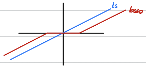
The result is totally different: \[ \hat w _i^{lasso}=sign(w _i^{ls})(w _i^{ls}-\lambda) _+ \] I draw a picture by hand to illustrate the difference.

What if we have a prior over \(W\) (Baysian way)

Model: \[ Y=XW+\epsilon \\ \epsilon \sim N(0,\sigma ^2)\\ W \sim Pr(W)\\ in \ this \ case \ we \ assume: \ W\sim N(0,\sigma _0^2) \]

\[ \begin{equation}\begin{split} \hat W^{MAP} &=argmax_Wln \ p(W|Y)\\ &=argmax_Wln \ \frac{p(Y|W)p(W)}{p(Y)}\\ &=argmax_Wln \ p(Y|W)p(W)\\ &=argmax_Wln \ \frac{1}{\sqrt{2\pi}\sigma}exp(-\frac{(y _i-W^Tx _i)^2}{2\sigma ^2})\frac{1}{\sqrt{2\pi}\sigma_0}exp(-\frac{||W||^2}{2\sigma _0^2})\\ &=argmin_W\sum _{i=1}^N\frac{(y _i-W^Tx _i)^2}{2\sigma ^2}+\frac{||W||^2}{2\sigma _0^2}\\ &=argmin_W\sum _{i=1}^N(y _i-W^Tx _i)^2+\frac{\sigma ^2}{\sigma _0^2}||W||^2 \end{split}\end{equation} \]

The next part is same with MLE with ridge regularization.

You Will Find:

\[ Linear \ Square \ Method\\ \Leftrightarrow Maximum \ Likelihood \ Estimate \ (with \ guassian \ noise) \]

\[ Regularized \ Maximum \ Likelihood \ Estimate \\ \Leftrightarrow Maximum \ a \ posteriori \ estimation \ (with \ guassian \ prior \ over \ W) \]